|
Biodiversity Data Journal :
Data Paper (Biosciences)
|
|
Corresponding author: Anne S. Philippe (annephilippe9@gmail.com)
Academic editor: Sarah Faulwetter
Received: 25 Aug 2016 | Accepted: 09 Jan 2017 | Published: 12 Jan 2017
© 2017 Anne Philippe, Christine Plumejeaud-Perreau, Jérôme Jourde, Philippe Pineau, Nicolas Lachaussée, Emmanuel Joyeux, Frédéric Corre, Philippe Delaporte, Pierrick Bocher
This is an open access article distributed under the terms of the Creative Commons Attribution License (CC BY 4.0), which permits unrestricted use, distribution, and reproduction in any medium, provided the original author and source are credited.
Citation:
Philippe A, Plumejeaud-Perreau C, Jourde J, Pineau P, Lachaussée N, Joyeux E, Corre F, Delaporte P, Bocher P (2017) Building a database for long-term monitoring of benthic macrofauna in the Pertuis-Charentais (2004-2014). Biodiversity Data Journal 5: e10288. https://doi.org/10.3897/BDJ.5.e10288
|
|
Abstract
Background
Long-term benthic monitoring is rewarding in terms of science, but labour-intensive, whether in the field, the laboratory, or behind the computer. Building and managing databases require multiple skills, including consistency over time as well as organisation via a systematic approach. Here, we introduce and share our spatially explicit benthic database, comprising 11 years of benthic data. It is the result of intensive benthic sampling that has been conducted on a regular grid (259 stations) covering the intertidal mudflats of the Pertuis-Charentais (Marennes-Oléron Bay and Aiguillon Bay). Samples were taken by foot or by boats during winter depending on tidal height, from December 2003 to February 2014. The present dataset includes abundances and biomass densities of all mollusc species of the study regions and principal polychaetes as well as their length, accessibility to shorebirds, energy content and shell mass when appropriate and available. This database has supported many studies dealing with the spatial distribution of benthic invertebrates and temporal variations in food resources for shorebird species as well as latitudinal comparisons with other databases. In this paper, we introduce our benthos monitoring, share our data, and present a "guide of good practices" for building, cleaning and using it efficiently, providing examples of results with associated R code.
New information
The dataset has been formatted into a geo-referenced relational database, using PostgreSQL open-source DBMS. We provide density information, measurements, energy content and accessibility of thirteen bivalve, nine gastropod and two polychaete taxa (a total of 66,620 individuals) for 11 consecutive winters. Figures and maps are provided to describe how the dataset was built, cleaned, and how it can be used. This dataset can again support studies concerning spatial and temporal variations in species abundance, interspecific interactions as well as evaluations of the availability of food resources for small- and medium size shorebirds and, potentially, conservation and impact assessment studies.
Keywords
Intertidal mudflats, benthic macrofauna, annelids, molluscs, monitoring, Pertuis-Charentais, shorebirds, database management
Introduction
Genesis: This benthos monitoring was initiated in winter 2003-2004 with the aim of describing feeding resources for overwintering shorebird species (e.g. Curlews, Grey Plovers, Bar-tailed Godwits, Black-tailed Godwits, Red knots, Dunlins, Oystercatchers, Redshanks and one duck species: Shelducks). At first, spatial studies were initiated and led to reference papers in ecosystem comparisons in the domain of molluscan studies (
Objectives: The initial purpose of the monitoring was to study the spatio-temporal variations of main macrobenthic species as available resources for shorebirds. Knowing individuals to the species level, their length, shell mass, accessibility (the top fraction was analysed separately) and flesh energy content, one can analyse for example:
- the spatial variability of densities of benthos prey, including comparisons with other countries (
Bocher et al. 2007 ); - the fraction available for Calidris canutus and Calidris alpina (sandpiper species), since the top 4 cm of the cores were analysed separately and shells were measured (
Philippe et al. 2016 ); - based on the quality of the molluscs (flesh to shell ratio) it is possible to predict the diets of red knots Calidris canutus using a digestive rate model derived from type II functional response curve, depending on the site and the year (
van Gils et al. 2004 Quaintenne et al. 2011 ).
Project description
Long-term molluscs and annelids monitoring in the Pertuis-Charentais, France
The monitoring was conducted every year under the responsibility of Pierrick Bocher with constant participation of Philippe Pineau and Nicolas Lachaussée and managers of the National Nature Reserves of Aiguillon Bay and Marennes-Oléron Bay. Additional help in the field was provided by multiple other colleagues and PhD candidates throughout the years.
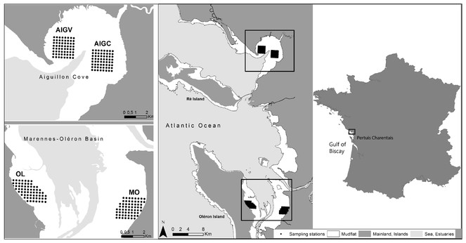
Sampling was performed on intertidal mudflats located in national nature reserves: RNN Aiguillon Bay and RNN Moëze-Oléron.
Systematic sampling was performed on four regular 250 m grids, composed of 64 stations each (except for the subsite "Oléron" (OL) which contained 67 stations).
The monitoring was funded by the University of La Rochelle and the CNRS via laboratory donations and staff time. Financial support was received from the Région Poitou-Charentes through a thesis grant to Anne Philippe (2013-2016). LIENSs laboratory and the DYFEA team also provided help with field work costs. The Office National de la Chasse et de la Faune Sauvage (ONCFS) and the Ligue pour la Protection des Oiseaux (LPO) supported this monitoring via staff time and nautical resources dedicated to sample collections.
Sampling methods
Benthic macrofauna was collected over a predetermined 250 m grid following a proven sampling protocol (
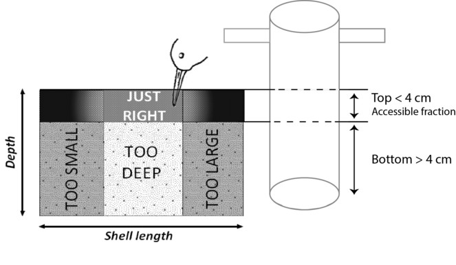
The harvestable fraction corresponding to the mean bill length of the sandpipers, the dunlin Calidris alpina and the red knot Calidris canutus and composed of the accessible fraction of benthos (found in the top 4 cm of the mud core) and of ingestible sizes (not too large and not too small). Ingestible sizes are species specific, and depend on the shape of the mollusc. Sizes available for C. canutus and C. alpina species are reported in
The cores were sieved through a 1 mm mesh, except for the mudsnail H. ulvae cores, which were sieved over a 0.5 mm mesh to prevent the loss of individuals smaller than 1mm (from the apex to the aperture). All living molluscs were collected in plastic bags and frozen (-18°C) until laboratory treatment (Fig.
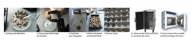
Sample processing: In the laboratory, molluscs were identified under the supervision of a benthic taxonomist. Individuals were counted, and their maximum length was measured to the nearest 0.1 mm using Vernier calipers, width was also measured for bivalves. Hydrobiid mudsnails were size-categorised from 0 mm up to 6 mm (e.g. size class 2 consisted of individuals with lengths ranging from 2 to 2.99 mm).
The flesh of every mollusc specimen except H. ulvae was detached from the shell and placed individually in crucibles (pooled by size class when sizes were smaller than 8.0 mm, flesh and shell together). Crucibles containing molluscs were placed in a ventilated oven at 55 to 60°C for three days until constant mass and then weighed (DM ±0.01 mg). Dried specimens were then incinerated at 550°C for 4 h to determine their ash mass and then a proxy of their energy content: the ash free dry mass (AFDM). [H. ulvae flesh biomass (AFDMflesh) was estimated for each station from the total biomass (AFDMflesh+shell) with the following linear regression: AFDMflesh= 0.6876 × AFDMflesh+shell + 7E-05 (R² = 0.99; N = 60 individuals sampled in July 2014 in Aiguillon Bay). Flesh biomass of bivalves (Scrobicularidae, as well as Macoma balthica individuals) smaller than 8.0 mm was determined from the total biomass (AFDMflesh+shell) with the following linear regression: AFDMflesh= 0.7649 × AFDMflesh+shell − 7E-05 (R² = 0,9656, N = 122 Scrobiculalidae individuals and 51 M. balthica ind. sampled in January 2014 in Aiguillon Bay).
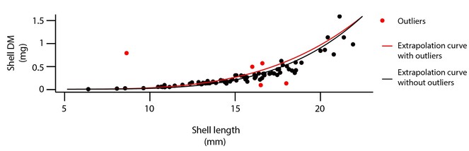
For bivalves larger than 8.0 mm, shells were placed in adequate numbered stalls and dried in a ventilated oven at 55 to 60°C (DM ±0.01 mg) for three days. For H. ulvae individuals, shell was not separated from the flesh, and shell dry mass was estimated from the total biomass using the following regression: DMshell = 5.5902 × AFDMflesh+shell – 0.0006 (R² = 0.98; N=60 ind. sampled in July 2014 in Aiguillon Bay). For the same reason, dry mass of the shell (DMshell) of small bivalves (< 8.0 mm) was extrapolated using the following regression: DMshell = 8E-05 × Length 2,6523 (R² = 0,8274, N=122 Scrobiculalidae ind. and 51 M. balthica ind. sampled in January 2014 in Aiguillon Bay).
In the present dataset, we removed all epibenthic species (e.g. crustaceans) since they are nearly absent from the feeding regime of shorebirds in our study area (
Geographic coverage
In winter 2003-2004, an extensive benthos sampling (864 stations) was conducted following a grid over the whole intertidal zone of Aiguillon Bay and Marennes-Oléron Bay (
Due to field complexities or bad weather, some stations were not sampled some years. Namely in 2004, stations 2131-2133 and 2136-2140; in 2006, stations 2103 and 1953; in 2005, stations 1860, 1391 and 1395; in 2008, station 1300; in 2010, station 1958; in 2012, station 2137; and in 2014, stations 2137 and 1311. To this list, all the stations from Marennes-Oléron (site 'OL' and 'MO') in years 2010 and 2011 should be added. The value “NA” (i.e. not available) is given in the data set to avoid misinterpreting these cases for true “absence”.
Taxonomic coverage
The dataset includes all occurrences of individuals for the taxa listed in Table
Table of attributes, with associated column names, description, units and constraints in the benthos dataset.
| Attribute | Column_name | Description | Units | Constraints |
| AphiaID | AphiaID | Unique number corresponding to a described species in WoRMS | - | Integer |
| Period | "Period" | Winter period corresponding to the sampling | - | Text, ["Winter 2003-2004" to "Winter 2013-2014"] |
| Sampling date | "sampling_date" | Date of sampling | - | Datastyle, DMY format |
| Site | "site" | Sampling site | - | 'MAROL' refers to Marennes Oléron Bay, and 'AIG' refers to Aiguillon Bay |
| Subsite | "st_sit_id" | Subsite | - | Each site is divided into two subsites (grids of approximately 64 stations). Oléron subsite ('ol') and Moëze subsite ('mo') are part of the site 'MAROL'. Aiguillon Charente subsite ('aic') and Aiguillon Vendée subsite ('aiv') are part of the site 'AIG'. |
| Station | "Poskey" | Station number | - | Each station refers to unique coordinates ("st_lat_dd" and "st_long_dd") and is located in a single "site" and "subsite". Subsite 'ol' has 67 stations, and subsites 'mo', 'aic' and 'aiv' have 64 |
| Latitude | "st_lat_dd" | Latitude | Decimal degrees, WGS84 | Numeric, together with "st_long_dd" refer to a single "Poskey" value |
| Longitude | "st_long_dd" | Longitude | Decimal degrees, WGS84 | Numeric, together with "st_lat_dd" refer to a single "Poskey" value |
| Number | "number" | Number of individual | - | Integer = 1 |
| Shell length | "length" | Maximum length of the shell | mm | Numeric, decimal = 2. 'NA' when "Phylum" is 'Annelida'. Measured from the apex to the aperture when Gastropoda. Measured as the maximum length of the shell when Bivalve. For the species 'hyd', length is rounded to the closest lower integer |
| Size class | "class_length" | Size class of the individual | mm | Integer, corresponded to the "length" value, rounded to the closest integer |
| Shell width | "width" | Width of the bivalve | mm | Numerical, decimal = 2, only measured for bivalves as the maximum width when both valves are taken together |
| Flesh AFDM | "AFDM" | Ash-Free Dry Mass of the soft part | g | Numerical, decimal = 4. 'NA' when "Phylum" is 'Annelida' |
| Shell DM | "ShellDM" | Dry mass of the shell | g | Numerical, decimal = 4. 'NA' when "Phylum" is 'Annelida' |
| Sampling mode | "car_mod_id" | Sampling mode, either by boat or by foot | _ | Integer, value in (1,2). If sampling was made by foot "car_mod_id" = 1. If sampling was made from boats "car-mod_id" = 2 |
| Accessibility | "car_top_bottom" | Whether or not the top 4 cm were seperated from the rest of the mud core | _ | Logical, if "car_mod_id" = 1 then "car_top_bottom" = TRUE |
| Sediment layer | "T.B.H" | Type of corer used | _ | Integer, value in ('top','bott','hyd','all'). If "car_mod_id" = 1, then "T.B.H" = 'hyd' if "abr" is 'hyd' otherwise if the individual is a different species of mollusc "T.B.H" = 'top' or 'bott' depending on the mud layer processed. If "car_mod_id" = 2 OR "Phylum" = 'Annelida' then "T.B.H" = 'all'. |
| Extrapolated Accessibility | "newTBH" | Extrapolated value, from the column "T.B.H" | _ | Character, value in ('t', 'b'), for other constraints see section "Cleaning process" and the paragraph "Extrapolating top and bottom fractions" of the present article |
| Sampled area | "area" | Sampled area, corresponding to the individual | m² | Numerical, decimal = 8. If "T.B.H" is 'top' or 'bott' then diameter of the corer is 7.5 cm and area = PI X 0,075². If "T.B.H" is 'hyd' then a smaller corer was used with a 3.5 cm diamater and area= PI X 0,035². If "T.B.H" is 'all' and "car_mod_id" is 1 then area = PI X 0,075². If "T.B.H" is 'all' and "car_mod_id" is 2 then two cores of 10 cm diameter were taken and area = 2 X PI X 0,100² |
| Abundance density | "dens.ind" | Abundance density | m-2 | Numerical, decimal = 4. "number" / "area" |
| Biomass density | "biomass.dens" | Density of flesh Ash-Free Dry Mass | g.m-2 | Numerical, decimal = 4. "AFDM" / "area" |
| Scientific name | "scientific_name" | Scientific name of the species | - | Binomial nomenclature |
| Phylum | "phylum" | Phylum of the sampled individual | - | Character, value in ('Annelida', 'Mollusca') |
| Class | "class" | Class associated to the individual | - | Text, according to WoRMS |
| Family | "family" | Family associated to the individual | Text, according to WoRMS | |
| Genus | "genus" | Genus associated to the indivual | - | Text, according to WoRMS |
| English common name | "English name" | English common name associated with the individual | - | Text, according to WoRMS |
| Authority | "authority" | The person credited to have formally named the species for the first time | - | Text, parentheses if the original name of the species has changed |
| Number of individuals | "nr" | Total individuals of this species in the database | - | Integer |
Species collected, including total number of specimens in the database, and classification according to the World Register of Marine Species
| AphiaID | Scientific name | Class | Family | Genus | Common name | Authority | Nr. of specimens |
| 141435 | Abra nitida | Bivalvia | Semelidae | Abra | (Müller, 1776) | 23 | |
| 146467 | Abra ovata | Bivalvia | Semelidae | Abra | (Philippi, 1836) | 3 | |
| 138474 | Abra sp. | Bivalvia | Semelidae | Abra | Lamarck, 1818 | 10 | |
| 141439 | Abra tenuis | Bivalvia | Semelidae | Abra | (Montagu, 1803) | 3,726 | |
| 138998 | Cerastoderma edule | Bivalvia | Cardiidae | Cerastoderma | Edible cockle, common cockle | (Linnaeus, 1758) | 1,697 |
| 139410 | Corbula gibba | Bivalvia | Corbulidae | Corbula | European clam, Basket shell | (Olivi, 1792) | 1 |
| 138963 | Crepidula fornicata | Gastropoda | Calyptraeidae | Crepidula | Common Atlantic slippersnail | (Linnaeus, 1758) | 56 |
| 876816 | Tritia neritea | Gastropoda | Nassariidae | Tritia | Cyclope | (Linnaeus, 1758) | 42 |
| 146905 | Epitonium clathrus | Gastropoda | Eulimidae | Epitonium | European wentletrap | (Linnaeus, 1758) | 1 |
| 140656 | Crassostrea gigas | Bivalvia | Ostreidae | Crassostrea | Pacific oyster | (Thunberg, 1793) | 1 |
| 140074 | Haminoea hydatis | Gastropoda | Haminoeidae | Haminoea | (Linnaeus, 1758) | 55 | |
| 140126 | Hydrobia ulvae | Gastropoda | Hydrobiidae | Hydrobia | Mudsnail, laver spire shell | (Pennant, 1777) | 45,796 |
| 140262 | Littorina littorea | Gastropoda | Littorinidae | Littorina | Common periwinkle | (Linnaeus, 1758) | 38 |
| 140264 | Littorina saxatalis | Gastropoda | Littorinidae | Littorina | black-lined periwinkle | (Olivi, 1792) | 8 |
| 141579 | Macoma balthica | Bivalvia | Tellinidae | Macoma | Baltic tellin | (Linnaeus, 1758) | 3,930 |
| 140380 | Kurtiella bidentata | Bivalvia | Montacutidae | Kurtiella | (Montagu, 1803) | 20 | |
| 140480 | Mytilus edulis | Bivalvia | Mytilidae | Mytilus | Blue mussel | Linnaeus, 1758 | 11 |
| 138235 | Nassarius sp. | Gastropoda | Nassariidae | Nassarius | Duméril, 1805 | 2 | |
| 22496 | Nereididae indet. | Polychaeta | Nereididae | Blainville, 1918 | 1,151 | ||
| 129370 | Nepthys sp. | Polychaeta | Nephtyidae | Nephtys | Cuvier, 1817 | 1,648 | |
| 140589 | Nucula nitidosa | Bivalvia | Nuculidae | Nucula | Winckworth, 1930 | 1 | |
| 141134 | Retusa obtusa | Gastropoda | Retusidae | Retusa | Arctic barrel-bubble | (Montagu, 1803) | 148 |
| 141424 | Scrobicularia plana | Bivalvia | Semelidae | Scrobicularia | Peppery furrow shell | (da Costa, 1778) | 7,592 |
| 231748 | Ruditapes sp. | Bivalvia | Veneridae | Ruditapes | Chiamenti, 1900 | 660 |
Traits coverage
The attributes of the database, including the traits measured in macrofauna individuals are presented in Table
Temporal coverage
Sampling was undertaken during winter (between December and February) each year, starting in December 2003. The fieldwork team (about five to seven people) spent a yearly average of three weeks per year sampling during spring tides in winter season. For convenience in analyses, if sampling took place in December, the year associated with sampling corresponds with the following year in the dataset. For example samples taken in December 2006 will be attached to year 2007, together with samples from January 2007 or February 2007. First samples were taken in December 2003 (sampling year 2004) and last samples in this database in February 2014 (year 2014). In the subsequent years (starting in winter 2015 until now) sampling was performed over a reduced spatial extent (only 'AIC' subsite, i.e. 64 stations). Sampling is planned to be continued in the future. The winter season was chosen because environmental conditions are stable for benthos (with a reduced growth rate and no recruitment for most species). Also, this is the period when the highest densities of overwintering migratory shorebirds can be observed and can be linked to the feeding resources thanks to the annual January counts of Wetlands international. No data is available for the subsites 'mo' and 'ol' in sampling years 2010 and 2011.
Usage rights
This work is licensed under a Creative Commons Attribution-NonCommercial-ShareAlike 4.0 International License. The associated dataset can be freely used for non-commercial purpose, provided it is cited. We draw your attention to the fact that you can contact the authors of the "benthos" dataset to prevent any misuse of the data. You can also consult us for reviewing articles based on our dataset.
Data resources
This dataset is hosted by EurOBIS and can be downloaded using the link above (see section 'Usage rights' for more information). The column names used in the present dataset don not always match the ones in the EurOBIS dataset. The Table below indicates this correspondance between the column names in the datapaper (including the names used in the script) and the column names in the EurOBIS dataset.
| Column label | Column description |
|---|---|
| aphiaid | Unique number corresponding to a described species in WoRMS. In the present datapaper the column refers to the column 'AphiaID'. |
| period | Winter period corresponding to the sampling.In the present datapaper the column refers to the column 'Period'. |
| sampling_date | Date of sampling.In the present datapaper the column refers to the column 'sampling_date'. |
| site | Sampling site.In the present datapaper the column refers to the column 'site'. |
| st_sit_id | Subsite.In the present datapaper the column refers to the column 'st_sit_id'. |
| station | Station number.In the present datapaper the column refers to the column 'Poskey'. |
| st_lat_dd | Latitude.In the present datapaper the column refers to the column 'st_lat_dd'. |
| st_long_dd | Longitude.In the present datapaper the column refers to the column 'st_long_dd'. |
| number | Number of individual.In the present datapaper the column refers to the column 'number'. |
| length | Maximum length of the shell.In the present datapaper the column refers to the column 'length'. |
| class_length | Size class of the individual.In the present datapaper the column refers to the column 'class_length'. |
| width | Width of the bivalve.In the present datapaper the column refers to the column 'width'. |
| afdm | Ash-Free Dry Mass of the soft parts.In the present datapaper the column refers to the column 'AFDM'. |
| shelldm | Dry mass of the shell.In the present datapaper the column refers to the column 'ShellDM'. |
| car_mod_id | Sampling mode, either by boat or by foot.In the present datapaper the column refers to the column 'car_mod_id'. |
| car_top_bottom | Whether or not the top 4 cm were seperated from the rest of the mud core.In the present datapaper the column refers to the column 'car_top_bottom'. |
| tbh | Type of corer used.In the present datapaper the column refers to the column 'T.B.H'. |
| newtbh | Extrapolated value, from the column "T.B.H".In the present datapaper the column refers to the column 'newT.B.H'. |
| area | Sampled area, corresponding to the individual.In the present datapaper the column refers to the column 'area'. |
| dens.ind | Abundance density.In the present datapaper the column refers to the column 'dens.ind'. |
| biomass.dens | Density of flesh Ash-Free Dry Mass.In the present datapaper the column refers to the column 'biomass_dens'. |
| scientific_name | Scientific name of the species.In the present datapaper the column refers to the column 'Scientific name'. |
| phylum | Phylum of the sampled individual.In the present datapaper the column refers to the column 'phylum'. |
| class | Class associated with the individual.In the present datapaper the column refers to the column class'. |
| family | Family associated with the individual.In the present datapaper the column refers to the column 'family'. |
| genus | Genus associated with the individual.In the present datapaper the column refers to the column genus'. |
| English name | English common name associated with the individual.In the present datapaper the column refers to the column 'English name'. |
| authority | The person credited to have formally named the species for the first time.In the present datapaper the column refers to the column 'authority'. |
| nr | Total individuals of this species in the database.In the present datapaper the column refers to the column 'nr'. |
Additional information
Steps of database building
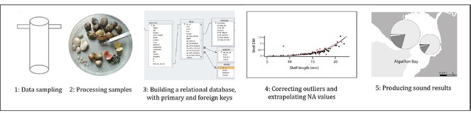
The dataset was built via the association of different original tables at different steps of the collection, sorting, measuring and weighing of samples. After each sampling session, we filled in a table "CORE" with columns: "year", "Poskey", "car_mod_id" and "car_top_bottom" as well as unique identifier "core_id". Subsequently, in the laboratory while determining and measuring the samples, we filled in a table "BENTHOS" with columns: "abr", "number", "length", "width", "class_length", "T.B.H", "AFDM", "Shell_DM" and "core_id". A unique idendifier "id" was associated to each row in this table "BENTHOS".
Preliminary to the tables "CORE" and "BENTHOS", a table "SPECIES" with the scientific name associated to the abbrevation "abr" was built, together with a table "STATIONS" with coordinates, site and subsite associated to the sampling station identifier "Poskey".
All these tables were associated together, in strict respect of integrity criteria specified through 'foreign keys' and 'primary keys' constraints, to form a relational database (Fig.
Cleaning process
Step 1. Check integrity constraints, misspellings, uniqueness: The preparation of the dataset (e.g. checking for data types, misspelling, uniqueness of identifiers and integrity constraints as described in Table 2) was performed through building the relational database under PostGreSQL, following the principles described in
| Step 1. Check integrity constraints, misspellings, uniqueness | |||||
|---|---|---|---|---|---|
| Attribute | Description | Modified | Total occurrence | % corrected | Criteria |
| "abr" | Species abbreviation | 148 | 66,620 | 0.22% | misspelling |
| "car_top_bottom" | Whether the top fraction of the sediment was sampled separately | 460 | 7,013 | 6.56% | logic |
| "AFDM" | Flesh ash-free dry mass | 2,215 | 11,015 | 20.11% | "length" > 8 |
| "ShellDM" | Shell dry mass | 2,353 | 11,015 | 21.36% | "length" > 8 |
| Step 2. Detect & remove outliers, infer missing values | |||||
| Attribute | Description | Modified | Total occurence | % corrected | Criteria |
| "length" | Length of the shell | 140 | 66,620 | 0.21% | "length" = 0 |
| "AFDM" | Flesh ash-free dry mass | 52,127 | 53,533 | 97.37% | "length" < 8 |
| "ShellDM" | Shell dry mass | 10,308 | 53,533 | 19.26% | "length" < 8 |
| "newTBH" | Whether the individual belongs to the top or the bottom (inferring) | 10,884 | 21,918 | 49.66% | probabilities |
Step 2. Outliers and NA, using regression models on data: Once the relational database was built, and integrity criteria met, the database was cleaned in a systematic way, species by species, site by site and year by year. This step was done using R statistical software (
Assigning sampling area to each station in each year, depending on the sampling method: The columns "area" and "area_hyd" were filled in according to the sampling method (either by boat "car_mod_id"= 2 or by foot "car_mod_id"=1). By boat, two cores are taken using a corer with a radius of 0.050 m (area= 2 x (PI x 0.050²)); by foot, one core was taken with radius of 0.075 m (area= PI x 0.075²). Hydrobia ulvae were counted in one of the two cores taken by boat (area= PI x 0.050²), and if sampling was made by foot an additional smaller core was taken, with a radius of 0.035 m (area= PI x 0.035²), see Table
Calculating abundance and biomass densities: The next step consisted of deriving abundance densities ("dens_ind") and biomass densities ("biomass_dens"), see Suppl. material
Extrapolating top and bottom fractions: The last step of data cleaning aimed at assigning the sampled individuals to the top or the bottom fraction of the sediment (i.e. whether or not it was accessible to a sandpiper's bill). When samples were taken by foot ("car_mod_id"=1), the top 4 cm were always separated from the bottom fraction ("car_top_bottom"=TRUE), and the sampled individuals always received a "top" or "bott" or "hyd" value in the column "T.B.H", "hyd" corresponding to the top fraction of the sediment since H. ulvae are always accessible to sandpipers. However, when samples were taken from boats ("car_mod_id"=2), the top was not separated from the bottom fraction ("car_top_bottom"=FALSE), and the sampled individuals did not receive a "top" or "bott" value in the column "T.B.H". In that case, a script (Suppl. material
Discussion
Opportunities: There are multiple examples of the potential uses of those data for further exploitation. The multidimensional dataset can be explored for various questions and following spatial or temporal dimension. For instance, in Fig.
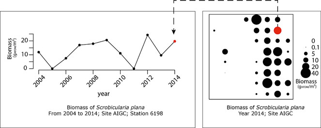
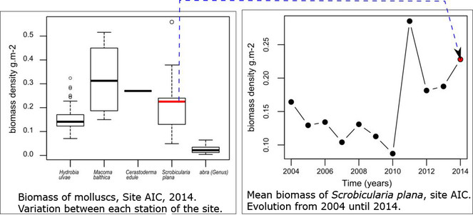
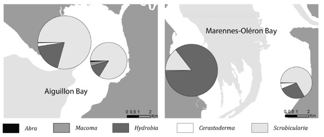
All the results presented in this datapaper can be obtained running the provided R code associated, see Suppl. material
Limits of data use: The data was designed to estimate temporal changes and spatial differences in biomass and densities, as well as possible changes in quality, depth or community composition in our study sites. However, for predictions at unsampled locations, additional analyses are required, such as investigating spatial auto-correlation (
Author contributions
Data collection, sorting and processing of samples as well as database integrity was initiated and managed by Dr. Pierrick Bocher (Senior Scientist at the LIENSs laboratory, University of La Rochelle) in 2003. One Assistant engineer (Philippe Pineau) and one technician (Nicolas Lachaussée) helped collecting the data every year. Anne Philippe helped in data collection, laboratory work, data uploading and was responsible for the design and integrity of the database. Transfer of the database into PostGreSQL format and preparation of the figures and scripts accompanying the present datapaper was performed by Dr. Christine Plumejeaud-Perreau (Research engineer at the LIENSs laboratory) with help from Anne Philippe. Jérôme Jourde was in charge of taxonomy training and helped with identification and cleaning of the database when necessary.
Contact: Dr Pierrick Bocher, Pierrick.Bocher@univ-lr.fr
Acknowledgements: Precious support in the field was provided by the staff of the Ligue pour la Protection des Oiseaux (LPO) and the Office National de la Chasse et de la Faune Sauvage (ONCFS), working in National Nature Reserves of the Region Poitou-Charentes (L. Jomat, S. Gueneteau, S. Haye and many others). We thank the managers of the National Nature Reserve of Aiguillon Bay, E. Joyeux and F. Corre and the manager of the National Nature Reserve of Moëze-Oléron P. Delaporte for their support and help. Sorting, identifying, measuring and weighing of benthic invertebrates were also the tasks of several interns and PhD candidates. Many colleagues from the laboratory helped occasionally: V. Huet regularly helped us with weighing samples and T. Guyot with sieving of cores. We also thank F. Robin for his large contribution to this database over several years. Adrien de Pierrepont (Bsc.) produced the extrapolation curves for H. ulvae shell dry mass and AFDM.
We would like to thank the reviewers of this datapaper, for their insightful comments and suggestions, as well as the editorial board for their reactivity throughout the reviewal process.
References
- Designing a benthic monitoring programme with multiple conflicting objectives.Methods in Ecology and Evolution3(3):526‑536. https://doi.org/10.1111/j.2041-210x.2012.00192.x
- Trophic resource partitioning within a shorebird community feeding on intertidal mudflat habitats.Journal of Sea Research92:115‑124. https://doi.org/10.1016/j.seares.2014.02.011
- Site- and species-specific distribution patterns of molluscs at five intertidal soft-sediment areas in northwest Europe during a single winter.Marine Biology151(2):577‑594. https://doi.org/10.1007/s00227-006-0500-4
- Principles and Methods of Data Cleaning - Primary Species and Species-Occurrence Data - version 1.0.GBIF,75pp. URL: http://www.gbif.org/orc/?doc_id=1262.
- Repeatable sediment associations of burrowing bivalves across six European tidal flat systems.Marine Ecology Progress Series382:87‑98. https://doi.org/10.3354/meps07964
- Comparative analysis of the food webs of two intertidal mudflats during two seasons using inverse modelling: Aiguillon Cove and Brouage Mudflat, France.Estuarine, Coastal and Shelf Science69:107‑124. https://doi.org/10.1016/j.ecss.2006.04.001
- Identification of outliers.11.Chapman and Hall,127pp.
- Handbook of the marine fauna of north-west Europe, xi, 800p. Oxford University Press, 1995.Journal of the Marine Biological Association of the United Kingdom76(1):264. https://doi.org/10.1017/s0025315400029301
- The role of environmental variables in structuring landscape-scale species distributions in seafloor habitats.Ecology91(6):1583‑1590. https://doi.org/10.1890/09-2040.1
- Landscape-scale experiment demonstrates that Wadden Sea intertidal flats are used to capacity by molluscivore migrant shorebirds.Journal of Animal Ecology78(6):1259‑1268. https://doi.org/10.1111/j.1365-2656.2009.01564.x
- Influence of environmental gradients on the distribution of benthic resources available for shorebirds on intertidal mudflats of Yves Bay, France.Estuarine, Coastal and Shelf Science174:71‑81. https://doi.org/10.1016/j.ecss.2016.03.013
- Scaling up ideals to freedom: are densities of red knots across western Europe consistent with ideal free distribution?Proceedings of the Royal Society B: Biological Sciences278(1719):2728‑2736. https://doi.org/10.1098/rspb.2011.0026
- Diet selection in a molluscivore shorebird across Western Europe: does it show short- or long-term intake rate-maximization?Journal of Animal Ecology79(1):53‑62. https://doi.org/10.1111/j.1365-2656.2009.01608.x
- R: A language and environment for statistical computing. R Foundation for Statistical Computing.Vienna, Austria.
- Digestive bottleneck affects foraging decisions in red knots Calidris canutus. I. Prey choice.Journal of Animal Ecology74(1):105‑119. https://doi.org/10.1111/j.1365-2656.2004.00903.x
- World Register of Marine Species, Webservice. http://www.marinespecies.org/aphia.php?p=webservice. Accessed on: 2016-10-20.
- World Register of Marine Species. http://www.marinespecies.org/index.php. Accessed on: 2016-10-20.
- WSDL interfcae, World Register of Marine Species. http://www.marinespecies.org/aphia.php?p=soap&wsdl=1. Accessed on: 2016-10-20.