|
Biodiversity Data Journal :
R Package
|
|
Corresponding author: Pedro Cardoso (pedro.cardoso@helsinki.fi)
Academic editor: Scott Chamberlain
Received: 23 Aug 2017 | Accepted: 17 Oct 2017 | Published: 19 Oct 2017
© 2017 Pedro Cardoso
This is an open access article distributed under the terms of the Creative Commons Attribution License (CC BY 4.0), which permits unrestricted use, distribution, and reproduction in any medium, provided the original author and source are credited.
Citation:
Cardoso P (2017) red - an R package to facilitate species red list assessments according to the IUCN criteria. Biodiversity Data Journal 5: e20530. https://doi.org/10.3897/BDJ.5.e20530
|
|
Abstract
The International Union for the Conservation of Nature Red List is the most useful database of species that are at risk of extinction worldwide, as it relies on a number of objective criteria and is now widely adopted. The R package red – IUCN Redlisting Tools - performs a number of spatial analyses based on either observed occurrences or estimated ranges. Functions include calculating Extent of Occurrence (EOO), Area of Occupancy (AOO), mapping species ranges, species distribution modelling using climate and land cover and calculating the Red List Index for groups of species. The package allows the calculation of confidence limits for all measures. Spatial data of species occurrences, environmental or land cover variables can be either given by the user or automatically extracted from several online databases. It outputs geographical range, elevation and country values, maps in several formats and vectorial data for visualization in Google Earth. Several examples are shown demonstrating the usefulness of the different methods. The red package constitutes an open platform for further development of new tools to facilitate red list assessments.
Keywords
Area of Occupancy, Extent of Occurrence, extinction risk, International Union for the Conservation of Nature, red list index, species distribution modelling
Introduction
The IUCN Red List of Threatened Species is the most widely used information source on species extinction risk (
For the vast majority of species that lack appropriate data on population size and decline (
The IUCN Red List Index (RLI) (
Following a series of tools that have been recently developed to facilitate species assessments, such as a specific type of peer-reviewed article that directly feeds into the IUCN Red List (
Specification
The R package red performs a number of spatial analyses based on either observed occurrences or estimated ranges. Importantly, given the frequent shortcomings of available data, the package allows the calculation of confidence limits for EOO, AOO and the RLI. It outputs geographical range, elevation and country values, maps in several formats and vector data for visualization in Google Earth. The package is written in R and can be installed from the Comprehensive R Archive Network (https://CRAN.R-project.org/package=red). The newest, often a development version, is also available at GitHub (https://github.com/cardosopmb/red). The raw data accepted by most functions are: 1) a matrix of longitude and latitude or eastness and northness of species occurrence records, and 2) a raster* object as defined by the R package raster (
Extent of Occurrence (eoo) - Calculates the EOO of a species based on either records or predicted distribution. EOO is calculated as the minimum convex polygon covering all known or predicted sites for the species.
Area of Occupancy (aoo) - Calculates the AOO of a species based on either known records or predicted distribution. AOO is calculated as the area of all known or predicted cells for the species. The resolution is 2x2km as required by IUCN.
Recorded distribution of species (map.points) - Mapping of all cells where the species is known to occur. To be used if either information on the species is very scarce (and it is not possible to model the species distribution) or, on the contrary, complete (and there is no need to model the distribution).
Species distribution of habitat specialists (map.habitat) - Mapping of all habitat patches where the species is known to occur. In many cases a species has a very restricted habitat and we generally know where it occurs. In such cases using the distribution of the known habitat patches may be enough to map the species.
Species distribution modelling (map.sdm) - Prediction of potential species distributions using maximum entropy (maxent). Builds maxent models (
Map of multiple species simultaneously (map.easy) - Single step for mapping multiple species distributions, with or without modeling. Outputs maps in asc, pdf and kml formats, plus a file with EOO, AOO and a list of countries where the species is predicted to be present.
Red List Index (rli) - Calculates the Red List Index (RLI) for a group of species. The IUCN Red List Index (RLI) (
Red List Index for multiple groups (rli.multi) - Calculates the Red List Index (RLI) for multiple groups of species simultaneously.
Sampled Red List Index (rli.sampled) - Calculates accumulation curve of confidence limits in sampled RLI. In many groups it is not possible to assess all species due to huge diversity and/or lack of resources. In such case, the RLI is estimated from a randomly selected sample of species - the Sampled Red List Index (SRLI;
Usage
I provide an example of a typical session using red. Start by loading the package and retrieving species records:
library(red)
data(red.records)
spRec = red.records
Ten unique records for Hogna maderiana (Walckenaer, 1837), a spider endemic to Madeira Island, have longitude and latitude data. Users can provide their own distribution data in either longitude/latitude (projected automatically to metric units) or any metric system such as UTM (in which case make sure that all data are in the same zone). One can calculate EOO and AOO (in km2) and extract information on the countries occupied:
eoo(spRec)
aoo(spRec)
countries(spRec)
For species whose records are known to be complete or at least depict their entire geographic range this is the basic information to be used in assessments. For further analyses a set of environmental layers are needed in raster format. These can be either: 1) user-provided, matching the species records data units, or 2) set up automatically by the package. The function red.setup will download worldclim (
data(red.layers)
spRaster <- red.layers
raster::plot(spRaster)
One of these is the elevation for the region that can be used to extract information on species altitudinal range:
altRaster <- spRaster[[3]]
raster::plot(altRaster)
points(spRec, pch = 19)
elevation(spRec, altRaster)
Note that one record is in the sea (Fig.
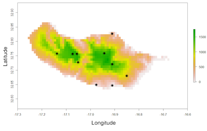
This may be due to spatial inaccuracy of the record or missing environmental data at the edges of the mainland or an island. In such cases, it might be good to move such points to the closest cell with environmental data:
spRec = move(spRec, spRaster)
points(spRec, pch = 19, col=“red”)
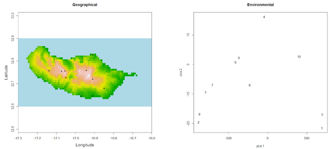
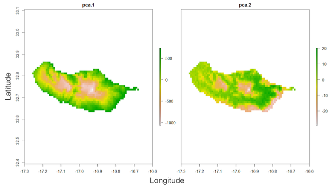
Unusual records can also be due to misidentifications, erroneous data sources or errors in transcriptions. These outliers can often be detected by looking at graphs of geographical or environmental space.
outliers(spRec, spRaster)
One might want to carefully look at records 1 and 5 (the ones at the southern coast of the island) as their environmental fingerprint is somewhat different from all other records as revealed by their distance to the centroid of the PCA (Fig.
It is now possible to attempt mapping the species distribution:
distrRaw <- map.points(spRec, spRaster)
Note that the output is a list with a raster depicting all the cells where the species is recorded and a second element with the respective values for EOO and AOO.
raster::plot(distrRaw[[1]])
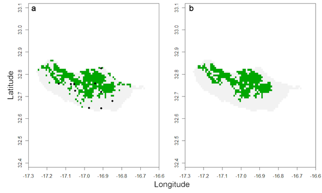
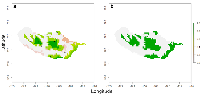
This map and values obviously assume that the records represent the entire range of the species. Yet, this is seldom true and in most cases some kind of extrapolation is justified. I propose two options within red to overcome the limitations of data. Often a species has a very restricted habitat and one generally knows where this habitat occurs. In such cases, using the distribution of the known habitat patches may be enough to accurately map the species. If one knows the spider species is currently restricted to forest areas:
spHabitat <- spRaster[[4]]
spHabitat[spHabitat != 4] <- 0
spHabitat[spHabitat == 4] <- 1
par(mfrow=c(1,2))
raster::plot(spHabitat, legend = FALSE)
points(spRec, pch = 19)
If one assumes the species does not currently occur outside forests that once occupied most of the island or in many of the small, isolated, forest patches, the following function retrieves only habitat patches known to be occupied:
distrHabitat <- map.habitat(spRec, spHabitat, move = FALSE)
raster::plot(distrHabitat[[1]], legend = FALSE)
The output is again a list with a raster depicting all the cells where the species is potentially present (Fig.
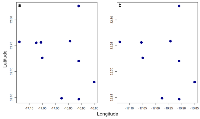
The second option available in red to overcome data deficiency is performing species distribution modelling (SDM) using Maxent (
plot(spRec, pch = 19)
thinRec <- thin(spRec, 0.1)
plot(thinRec, pch = 19)
In this case, no records are closer than 10% of the maximum distance between any two after thinning (Fig.
Overfitting is also a possibility in SDMs if the number of records is low compared to the number of predictor variables (environmental or other layers). The following function reduces the number of dimensions through either PCA or eliminating highly correlated layers:
spRaster <- raster.reduce(red.layers[[1:3]], n = 2)
raster::plot(spRaster)
Note that land use was not used as it is a categorical variable (Fig.
Only after all pre-processing of occurrence and climatic plus land use data is it possible to model the distribution. This example uses ensemble modelling (
spMap = map.sdm(spRec, spRaster, runs = 100)
raster::plot(spMap[[2]])
points(spRec, pch = 19)
raster::plot(spMap[[1]])
The consensus map (Fig.
IUCN requires maps to support the assessments, and red has the possibility of exporting them in several formats, namely kml:
par(mfrow = c(1,1))
map.draw(spRec, spMap[[1]])
kml(spMap[[1]], filename = "spMap.kml")
As an alternative or exploratory step, there is a function that performs most of this process in an automated way for multiple species (map.easy).
Finally, it is possible to calculate the Red List Index for single or multiple taxa simultaneously, including the calculation of confidence limits through bootstrapping:
rliData <- matrix(c("LC","LC","EN","EN","EX","EX","LC","CR","CR","EX"), ncol = 2, byrow = TRUE)
colnames(rliData) <- c("2000", "2010")
rli(rliData)
rliData <- cbind(c("Arthropods","Arthropods","Birds","Birds","Birds"), rliData)
rli.multi(rliData, boot = TRUE)
Discussion
Strengths
The red package allows a fully data-driven and transparent assessment process within the most used statistical software package in ecological sciences - R. The software is open-source and being continuously developed (https://github.com/cardosopmb/red). It contains numerous tools, including methods not available in any other package or software. These include calculating EOO and AOO following the IUCN guidelines based on habitat or species distribution modelling, exporting maps in both pdf and kml formats, extracting information on elevation range and countries occupied by the species and calculating various formulations of the Red List Index. Importantly, it is the only software available to calculate all quantitative measures (EOO, AOO, RLI) with confidence limits, allowing the assessor to take data uncertainty into account.
Caveats
Although red was specifically designed to be as simple to use as possible, as most IUCN assessors have little familiarity with R or programming in general, minimum skills are still required. It is also still lacking functions for many of the criteria, such as estimating past or future changes in EOO, AOO or population size (but see future developments below).
Alternatives
To my knowledge, three other R packages intended to help with Red List threat assessments have been released. rCAT (
Future developments
A number of developments are foreseen in red´s future. These include:
1. Calculating alpha-hulls for robust analysis of reductions or continuing declines in EOO (
2. Calculating the number of subpopulations and locations with a hint on fragmentation analysis.
3. Estimating past or future reductions in EOO and AOO based on dates of sampling records, land use/cover and climate change.
4. Incorporating phylogenetic and functional diversity information in RLI calculations.
5. Identifying candidate Key Biodiversity Areas (http://www.keybiodiversityareas.org).
The R package red tries to fill a gap in threat assessments according to the IUCN criteria using robust and replicable analytical methods. It is open source and any contributions to its continuous development are most welcome.
Citation
Researchers using red for publications should cite this article and in addition can also cite the red package directly. Updated citation information can be obtained by typing citation("red") in R.
Web location (URIs) and repository
Acknowledgements
Steven Bachman, Diogo Provete and Scott Chamberlain provided very useful comments that allowed improving the paper. PC and the IUCN SSC Spider & Scorpion Specialist Group are supported by Koneen Säätiö, the Mohamed Bin Zayed Species Conservation Fund, the Chicago Zoological Society CBOT Endangered Species Fund and Toyota Global Species Programme.
References
- spThin: an R package for spatial thinning of species occurrence records for use in ecological niche models.Ecography38(5):541‑545. https://doi.org/10.1111/ecog.01132
- Making consistent IUCN classifications under uncertainty.Conservation Biology14(4):1001‑1013. https://doi.org/10.1046/j.1523-1739.2000.99125.x
- Ensemble forecasting of species distributions.Trends in Ecology & Evolution22(1):42‑47. https://doi.org/10.1016/j.tree.2006.09.010
- Supporting Red List threat assessments with GeoCAT: geospatial conservation assessment tool.ZooKeys150:117‑126. https://doi.org/10.3897/zookeys.150.2109
- Toward monitoring global biodiversity.Conservation Letters1(1):18‑26. https://doi.org/10.1111/j.1755-263x.2008.00009.x
- Bias in species range estimates from minimum convex polygons: implications for conservation and options for improved planning.Animal Conservation6(1):19‑28. https://doi.org/10.1017/s1367943003003044
- Measuring global trends in the status of biodiversity: Red List Indices for birds.PLoS Biology2(12):e383. https://doi.org/10.1371/journal.pbio.0020383
- Improvements to the Red List Index.PloS One2(1):e140. https://doi.org/10.1371/journal.pone.0000140
- red: IUCN Redlisting Tools.1.2.1. URL: https://CRAN.R-project.org/package=red
- The seven impediments in invertebrate conservation and how to overcome them.Biological Conservation144(11):2647‑2655. https://doi.org/10.1016/j.biocon.2011.07.024
- Adapting the IUCN Red List criteria for invertebrates.Biological Conservation144(10):2432‑2440. https://doi.org/10.1016/j.biocon.2011.06.020
- Species Conservation Profiles compliant with the IUCN Red List of Threatened Species.Biodiversity Data Journal4:e10356. https://doi.org/10.3897/BDJ.4.e10356
- rredlist: 'IUCN' Red List Client.0.4.0. URL: https://github.com/ropensci/rredlist
- ConR: Computation of Parameters Used in Preliminary Assessment of Conservation Status.1.2.1. Release date:2017-6-13. URL: https://CRAN.R-project.org/package=ConR
- A statistical explanation of MaxEnt for ecologists.Diversity and Distributions17:43‑57.
- The Shuttle Radar Topography Mission.Reviews of Geophysics45:2004‑2004.
- WorldClim 2: new 1-km spatial resolution climate surfaces for global land areas.International Journal of Climatologyhttps://doi.org/10.1002/joc.5086
- The application of IUCN Red List Criteria at regional evels.Conservation Biology15(5):1206‑1212. https://doi.org/10.1046/j.1523-1739.2001.00112.x
- raster: Geographic Data Analysis and Modeling.2.5-8. Release date:2016-6-02. URL: https://CRAN.R-project.org/package=raster
- dismo: Species Distribution Modelling.1.1.4. Release date:2017-1-08. URL: https://CRAN.R-project.org/package=dismo
- IUCN Red List Categories and Criteria version 3.1. http://www. redlist.org/ technical-documents/categories-and-criteria/2001-categories-criteria. Accessed on: 2017-7-18.
- Trends of extinction risk for Lepidoptera in Finland: the first national Red List Index of butterflies and moths.Insect Conservation and Diversity9(2):118‑123. https://doi.org/10.1111/icad.12148
- Application of the Red List Index as an indicator of habitat change.Biodiversity and Conservation25(3):569‑585. https://doi.org/10.1007/s10531-016-1075-0
- redlistr: Tools for the IUCN Red List of Ecosystems and Species.1.0.0. Release date:2017-7-07. URL: https://CRAN.R-project.org/package=redlistr
- Assessing conservation status and trends for the world’s butterflies: the Sampled Red List Index approach.Journal of Insect Conservation15:121‑128. https://doi.org/10.1007/s10841-010-9329-8
- Quantification of extinction risk: IUCN's system for classifying threatened species.Conservation Biology22(6):1424‑1442. https://doi.org/10.1111/j.1523-1739.2008.01044.x
- The pitfall-trap of species conservation priority setting.Biodiversity and Conservation20(3):663‑682. https://doi.org/10.1007/s10531-010-9973-z
- rCAT: Conservation Assessment Tools.0.1.5. Release date:2017-1-17. URL: https://CRAN.R-project.org/package=rCAT
- Maximum entropy modeling of species geographic distributions.Ecological Modelling190:231‑259. https://doi.org/10.1016/j.ecolmodel.2005.03.026
- Maxent software for modeling species niches and distributions.3.4.1. URL: http://biodiversityinformatics.amnh.org/open_source/maxent
- The value of the IUCN Red List for conservation.Trends in Ecology & Evolution21:71‑76.
- The Barometer of Life.Science328:177‑177. https://doi.org/10.1126/science.1188606
- A global 1-km consensus land-cover product for biodiversity and ecosystem modelling.Global Ecology and Biogeography23(9):1031‑1045. https://doi.org/10.1111/geb.12182